Metrics reference - Lightdash

A metric is a value that describes or summarizes features from a collection of data points. For example: count of total number of user IDs, or sum of revenue. In Lightdash, metrics are used to summarize dimensions or, sometimes, other metrics.

Adding metrics to your project using the `meta` tag.

1. Using the column `meta` tag

To add a metric to Lightdash using the meta tag, you define it in your dbt project under the dimension name you’re trying to describe/summarize.

dbt v1.9 and earlier
dbt v1.10+ and Fusion
Lightdash YAML

models:
  - name: orders_model
    columns:
      - name: user_id # dimension your metric is aggregating
        meta:
          metrics:
            distinct_user_ids: # name of your metric
              type: count_distinct # metric type
      - name: revenue # dimension your metric is aggregating
        meta:
          metrics:
            sum_revenue: # name of your metric
              type: sum # metric type

models:
  - name: orders_model
    columns:
      - name: user_id # dimension your metric is aggregating
        config:
          meta:
            metrics:
              distinct_user_ids: # name of your metric
                type: count_distinct # metric type
      - name: revenue # dimension your metric is aggregating
        config:
          meta:
            metrics:
              sum_revenue: # name of your metric
                type: sum # metric type

type: model
name: orders_model

dimensions:
  - name: user_id # dimension your metric is aggregating
  - name: revenue # dimension your metric is aggregating

metrics:
  distinct_user_ids: # name of your metric
    type: count_distinct # metric type
    sql: ${TABLE}.user_id
  sum_revenue: # name of your metric
    type: sum # metric type
    sql: ${TABLE}.revenue

Once you’ve got the hang of what these metrics look like, read more about the metric types you can use below.

2. Using the model `meta` tag

Sometimes a metric references multiple columns, in these cases you can define the metric at the model level:

dbt v1.9 and earlier
dbt v1.10+ and Fusion
Lightdash YAML

models:
  - name: orders_model
    meta:
      metrics:
        revenue_per_user:
          type: number
          sql: ${sum_revenue} / ${distinct_user_ids}
        sum_total_paid:
          type: sum
          sql: ${revenue} + ${taxes_paid}

models:
  - name: orders_model
    config:
      meta:
        metrics:
          revenue_per_user:
            type: number
            sql: ${sum_revenue} / ${distinct_user_ids}
          sum_total_paid:
            type: sum
            sql: ${revenue} + ${taxes_paid}

type: model
name: orders_model

metrics:
  revenue_per_user:
    type: number
    sql: ${sum_revenue} / ${distinct_user_ids}
  sum_total_paid:
    type: sum
    sql: ${revenue} + ${taxes_paid}

Non-aggregate metrics (number, boolean, etc.) can only reference other metrics in sql: since they are inserted directly into the generated SQL query without being wrapped in an aggregate function.Aggregate metrics (sum, count_distinct, etc.) can only reference dimensions since they are wrapped in an aggregate function before being added to the generated SQL query. Wrapping an aggregate function in another aggregate function will cause an error.Post calculation metrics (percent_of_previous, percent_of_total, running_total) are computed after other metrics. They can reference aggregate and non-aggregate metrics only (they cannot reference dimensions or other post calculation metrics).

Read on to learn more about aggregate vs non-aggregate metrics!

Metric Categories

Each metric type falls into one of these categories. The metric categories tell you whether the metric type is an aggregation and what type of fields the metric can reference:

Aggregate metrics

Aggregate metric types perform (surprise, surprise) aggregations. Sums and averages are examples of aggregate metrics: they are measurements summarizing a collection of data points. Aggregate metrics can only reference dimensions, not other metrics.

Non-aggregate metrics

Non-aggregate metrics are metric types that, you guessed it, do not perform aggregations. Numbers and booleans are examples of non-aggregate metrics. These metric types perform a calculation on a single data point, so they can only reference aggregate metrics. They cannot reference dimensions.

Post calculation metrics

Post calculation metrics are computed after aggregate and non-aggregate metrics in the query. Because they run after the main aggregations, they can use window functions. Post calculation metrics:

Can only reference aggregate and non-aggregate metrics (they cannot reference dimensions or other post calculation metrics)
Can be referenced in table calculations like any other metric
Do not support the filters YML property

Experimental: Post calculation metrics are currently in the Experimental phase. Learn what this means in our Feature Maturity Levels guide: Feature Maturity Levels.

Metric configuration

You can customize your metrics in your dbt model’s YAML file. Here’s an example of the properties used in defining a metric:

dbt v1.9 and earlier
dbt v1.10+ and Fusion
Lightdash YAML

models:
  - name: sales_stats
    meta:
      joins:
        - join: web_sessions
          sql_on: ${web_sessions.date} = ${sales_stats.date}
      group_details:
        product_details:
          label: Product Details
          description: 'Fields that have information about the products in the basket.'
        item_details:
          label: Item Details
          description: 'Fields that have information about the items in the basket.'
    columns:
      - name: revenue
        description: 'Total estimated revenue in GBP based on forecasting done by the finance team.'
        meta:
          metrics:
            total_revenue:
              label: 'Total revenue GBP'
              type: SUM
              description: 'Total revenue in GBP'
              sql: 'IF(${revenue} IS NULL, 10, ${revenue})'
              groups: ['product_details', 'item_details'] # this would add the metric to a nested group: `product details` --> `item details`
              hidden: false
              format: '[$£]#,##0.00' # GBP rounded to two decimal points
              show_underlying_values:
                - revenue
                - forecast_date
                - web_sessions.session_id # field from joined table
              filters:
                - is_adjusted: true

models:
  - name: sales_stats
    config:
      meta:
        joins:
          - join: web_sessions
            sql_on: ${web_sessions.date} = ${sales_stats.date}
        group_details:
          product_details:
            label: Product Details
            description: 'Fields that have information about the products in the basket.'
          item_details:
            label: Item Details
            description: 'Fields that have information about the items in the basket.'
    columns:
      - name: revenue
        description: 'Total estimated revenue in GBP based on forecasting done by the finance team.'
        config:
          meta:
            metrics:
              total_revenue:
                label: 'Total revenue GBP'
                type: SUM
                description: 'Total revenue in GBP'
                sql: 'IF(${revenue} IS NULL, 10, ${revenue})'
                groups: ['product_details', 'item_details'] # this would add the metric to a nested group: `product details` --> `item details`
                hidden: false
                format: '[$£]#,##0.00' # GBP rounded to two decimal points
                show_underlying_values:
                  - revenue
                  - forecast_date
                  - web_sessions.session_id # field from joined table
                filters:
                  - is_adjusted: true

type: model
name: sales_stats

joins:
  - join: web_sessions
    sql_on: ${web_sessions.date} = ${sales_stats.date}

group_details:
  product_details:
    label: Product Details
    description: 'Fields that have information about the products in the basket.'
  item_details:
    label: Item Details
    description: 'Fields that have information about the items in the basket.'

dimensions:
  - name: revenue
    description: 'Total estimated revenue in GBP based on forecasting done by the finance team.'

metrics:
  total_revenue:
    label: 'Total revenue GBP'
    type: SUM
    description: 'Total revenue in GBP'
    sql: 'IF(${revenue} IS NULL, 10, ${revenue})'
    groups: ['product_details', 'item_details'] # this would add the metric to a nested group: `product details` --> `item details`
    hidden: false
    format: '[$£]#,##0.00' # GBP rounded to two decimal points
    show_underlying_values:
      - revenue
      - forecast_date
      - web_sessions.session_id # field from joined table
    filters:
      - is_adjusted: true

Here are all of the properties you can customize:

Property	Required	Value	Description
label	No	string	Custom label. This is what you’ll see in Lightdash instead of the metric name.
type	Yes	metric type	Metrics must be one of the supported types.
description	No	string	Description of the metric that appears in Lightdash. A default description is created by Lightdash if this isn’t included
sql	No	string	Custom SQL used to define the metric.
hidden	No	boolean	If set to true, the metric is hidden from Lightdash. By default, this is set to false if you don’t include this property.
compact	No	string	This option will compact the number value (e.g. 1,500 to 1.50K). Currently supports one of the following: [‘thousands’, ‘millions’, ‘billions’, ‘trillions’, ‘kilobytes’, ‘megabytes’, ‘gigabytes’, ‘terabytes’, ‘petabytes’, ‘kibibytes’, ‘mebibytes’, ‘gibibytes’, ‘tebibytes’, ‘pebibytes’]
format	No	string	This option will format the output value on the results table and CSV export. Supports spreadsheet-style formatting (e.g. #,##0.00). Use this website to help build your custom format.
separator	No	string	This option controls the grouping and decimal characters used when rendering numbers (e.g. `1.234.567,50` for European locales). One of: `default`, `commaPeriod`, `spacePeriod`, `periodComma`, `noSeparatorPeriod`, `apostrophePeriod`.
groups	No	string or string[]	If you set this property, the metric will be grouped in the sidebar with other metrics with the same group label.
urls	No	array	Adding urls to a metric allows your users to click metric values in the UI and take actions, like opening an external tool with a url, or open at a website. You can use liquid templates to customise the link based on the value of the dimension.
richText	No	string	Rich text template for displaying formatted content in table cells. Supports Markdown, HTML, and LiquidJS templating.
show_underlying_values	No	Array of dimension names	You can limit which dimensions or metrics are shown for a field when a user clicks View underlying data. The list must only include dimension/metric names from the base model or from any joined models. If not defined, we show all model dimensions.
filters	No	array	You can add filter logic to limit the values included in the metric calculation. You can add many filters. See which filter types are supported here.
tags	No	string[]	An array of string tags for categorizing and filtering metrics programmatically. Tags can be used by AI agents, API filters, and other backend workflows. See tags.

Metric types

Type	Category	Description
percentile	Aggregate	Generates a percentile of values within a column
median	Aggregate	Generates the 50th percentile of values within a column
average	Aggregate	Generates an average (mean) of values within a column
boolean	Non-aggregate	For fields that will show if something is true or false
count	Aggregate	Counts the total number of values in the dimension
count_distinct	Aggregate	Counts the total unique number of values in the dimension
date	Non-aggregate	For adding calculations to metrics that return dates.
max	Aggregate	Generates the maximum value within a numeric column
min	Aggregate	Generates the minimum value within a numeric column
number	Non-aggregate	For adding calculations to metrics that return numbers.
string	Non-aggregate	For metrics that contain letters or special characters
sum	Aggregate	Generates a sum of values within a column
sum_distinct	Aggregate (Beta)	Generates a sum of values, deduplicating by specified keys
average_distinct	Aggregate (Beta)	Generates an average of values, deduplicating by specified keys
percent_of_previous	Post calculation (Experimental)	Current value as a percentage of the previous row’s value
percent_of_total	Post calculation (Experimental)	Current value as a percentage of the total across the result set (or partition)
running_total	Post calculation (Experimental)	Cumulative total

percentile

Takes the percentile of the values in the given field. Like SQL’s PERCENTILE_CONT function. The percentile metric can be used on any numeric dimension or, for custom SQL, any valid SQL expression that gives a numeric table column. For example, this creates a metric median_price by taking the 50% percentile of the item_price dimension:

dbt v1.9 and earlier
dbt v1.10+ and Fusion
Lightdash YAML

columns:
  - name: item_price
    meta:
      metrics:
        median_price:
          type: percentile
          percentile: 50

columns:
  - name: item_price
    config:
      meta:
        metrics:
          median_price:
            type: percentile
            percentile: 50

type: model
name: my_model

dimensions:
  - name: item_price

metrics:
  median_price:
    type: percentile
    percentile: 50
    sql: ${TABLE}.item_price

median

Takes the 50th percentile of the values in the given field. Like SQL’s PERCENTILE_CONT(0.5) function. The median metric can be used on any numeric dimension or, for custom SQL, any valid SQL expression that gives a numeric table column. For example, this creates a metric median_price by taking the 50% percentile of the item_price dimension:

dbt v1.9 and earlier
dbt v1.10+ and Fusion
Lightdash YAML

columns:
  - name: item_price
    meta:
      metrics:
        median_price:
          type: median

columns:
  - name: item_price
    config:
      meta:
        metrics:
          median_price:
            type: median

type: model
name: my_model

dimensions:
  - name: item_price

metrics:
  median_price:
    type: median
    sql: ${TABLE}.item_price

average

Takes the average (mean) of the values in the given field. Like SQL’s AVG function. The average metric can be used on any numeric dimension or, for custom SQL, any valid SQL expression that gives a numeric table column. For example, this creates a metric avg_price by taking the average of the item_price dimension:

dbt v1.9 and earlier
dbt v1.10+ and Fusion
Lightdash YAML

columns:
  - name: item_price
    meta:
      metrics:
        avg_price:
          type: average

columns:
  - name: item_price
    config:
      meta:
        metrics:
          avg_price:
            type: average

type: model
name: my_model

dimensions:
  - name: item_price

metrics:
  avg_price:
    type: average
    sql: ${TABLE}.item_price

boolean

Tells you whether something is True or False. The boolean metric can be used on any valid SQL expression that gives you a TRUE or FALSE value. It can only be used on aggregations, which means either aggregate metrics or custom SQL that references other metrics. You cannot build a boolean metric by referencing other unaggregated dimensions from your model. boolean metrics don’t do any aggregations; they just reference other aggregations. For example, the avg_price metric below is an average of all of the item_price values in our product table. A second metric called is_avg_price_above_20 is a boolean type metric. The is_avg_price_above_20 metric has a custom SQL expression that tells us whether the avg_price value is greater than 20.

dbt v1.9 and earlier
dbt v1.10+ and Fusion
Lightdash YAML

columns:
  - name: item_price
    meta:
      metrics:
        avg_price:
          type: average
        is_avg_price_above_20:
          type: boolean
          sql: 'IF(${avg_price} > 20, TRUE, FALSE)'

columns:
  - name: item_price
    config:
      meta:
        metrics:
          avg_price:
            type: average
          is_avg_price_above_20:
            type: boolean
            sql: 'IF(${avg_price} > 20, TRUE, FALSE)'

type: model
name: my_model

dimensions:
  - name: item_price

metrics:
  avg_price:
    type: average
    sql: ${TABLE}.item_price
  is_avg_price_above_20:
    type: boolean
    sql: 'IF(${avg_price} > 20, TRUE, FALSE)'

count

Does a table count, like SQL’s COUNT function. The count metric can be used on any dimension or, for custom SQL, any valid SQL expression that gives a set of values. For example, this creates a metric number_of_users by counting the number of user_id values in the table:

dbt v1.9 and earlier
dbt v1.10+ and Fusion
Lightdash YAML

columns:
  - name: user_id
    meta:
      metrics:
        number_of_users:
          type: count

columns:
  - name: user_id
    config:
      meta:
        metrics:
          number_of_users:
            type: count

type: model
name: my_model

dimensions:
  - name: user_id

metrics:
  number_of_users:
    type: count
    sql: ${TABLE}.user_id

count_distinct

Counts the number of distinct values in a given field. It’s like SQL’s COUNT DISTINCT function. The count_distinct metric can be used on any dimension or, for custom SQL, any valid SQL expression that gives a set of values. For example, this creates a metric number_of_unique_users by counting the number of unique user_id values in the table:

dbt v1.9 and earlier
dbt v1.10+ and Fusion
Lightdash YAML

columns:
  - name: user_id
    meta:
      metrics:
        number_of_unique_users:
          type: count_distinct

columns:
  - name: user_id
    config:
      meta:
        metrics:
          number_of_unique_users:
            type: count_distinct

type: model
name: my_model

dimensions:
  - name: user_id

metrics:
  number_of_unique_users:
    type: count_distinct
    sql: ${TABLE}.user_id

date

Gives you a date value from an expression. The date metric can be used on any valid SQL expression that gives you a date value. It can only be used on aggregations, which means either aggregate metrics or custom SQL that references other metrics. You cannot build a date metric by referencing other unaggregated dimensions from your model. Creating a max or min date metric with type: date If you want to create a metric of a maximum or minimum date, you can’t use type: max or of type: min metrics because these are only compatible with numeric type fields. Instead, you can calculate a maximum or minimum date by defining a metric of type: date and using some custom sql, like this:

dbt v1.9 and earlier
dbt v1.10+ and Fusion
Lightdash YAML

columns:
  - name: created_at_date
    meta:
      dimension:
        type: date
      metrics:
        max_created_at_date:
          type: date
          sql: MAX(${TABLE}.created_at_date)

columns:
  - name: created_at_date
    config:
      meta:
        dimension:
          type: date
        metrics:
          max_created_at_date:
            type: date
            sql: MAX(${TABLE}.created_at_date)

type: model
name: my_model

dimensions:
  - name: created_at_date
    type: date

metrics:
  max_created_at_date:
    type: date
    sql: MAX(${TABLE}.created_at_date)

max

Max gives you the largest value in a given numeric field. It’s like SQL’s MAX function. The max metric can be used on any numeric dimension or, for custom SQL, any valid SQL expression that gives a numeric value. Because type: max metrics only work with numerical fields, you can’t use them to find a maximum date. Instead, you can use the MAX() function in the sql parameter of a metric of type: date to get a maximum date (you can see an example of this in the date section. For example, this creates a metric max_delivery_cost by looking at the delivery_cost dimension and taking the largest value it finds:

dbt v1.9 and earlier
dbt v1.10+ and Fusion
Lightdash YAML

columns:
  - name: delivery_cost
    meta:
      metrics:
        max_delivery_cost:
          type: max

columns:
  - name: delivery_cost
    config:
      meta:
        metrics:
          max_delivery_cost:
            type: max

type: model
name: my_model

dimensions:
  - name: delivery_cost

metrics:
  max_delivery_cost:
    type: max
    sql: ${TABLE}.delivery_cost

min

Min gives you the smallest value in a given numeric field. It’s like SQL’s MIN function. The min metric can be used on any numeric dimension or, for custom SQL, any valid SQL expression that gives a numeric value. Because type: min metrics only work with numerical fields, you can’t use them to find a minimum date. Instead, you can use the MIN() function in the sql parameter of a metric of type: date to get a minimum date (you can see an example of this in the date section. For example, this creates a metric min_delivery_cost by looking at the delivery_cost dimension and taking the smallest value it finds:

dbt v1.9 and earlier
dbt v1.10+ and Fusion
Lightdash YAML

columns:
  - name: delivery_cost
    meta:
      metrics:
        min_delivery_cost:
          type: min

columns:
  - name: delivery_cost
    config:
      meta:
        metrics:
          min_delivery_cost:
            type: min

type: model
name: my_model

dimensions:
  - name: delivery_cost

metrics:
  min_delivery_cost:
    type: min
    sql: ${TABLE}.delivery_cost

number

Used with numbers or integers. A number metric doesn’t perform any aggregation but can be used to perform simple transformations on other metrics. The number metric can be used on any valid SQL expression that gives you a numeric or integer value. It can only be used on aggregations, which means either aggregate metrics or custom SQL that references other metrics. You cannot build a number metric by referencing other unaggregated dimensions from your model. For example, this creates a metric called total_gross_profit_margin_percentage based on the total_sale_price and total_gross_profit_margin aggregate metrics:

dbt v1.9 and earlier
dbt v1.10+ and Fusion
Lightdash YAML

columns:
  - name: sale_price
    meta:
      metrics:
        total_sale_price:
          type: sum
  - name: gross_profit_margin
    meta:
      metrics:
        total_gross_profit_margin:
          type: sum
        total_gross_profit_margin_percentage:
          type: number
          sql: '(${total_gross_profit_margin}/ NULLIF(${total_sale_price},0))'

columns:
  - name: sale_price
    config:
      meta:
        metrics:
          total_sale_price:
            type: sum
  - name: gross_profit_margin
    config:
      meta:
        metrics:
          total_gross_profit_margin:
            type: sum
          total_gross_profit_margin_percentage:
            type: number
            sql: '(${total_gross_profit_margin}/ NULLIF(${total_sale_price},0))'

type: model
name: my_model

dimensions:
  - name: sale_price
  - name: gross_profit_margin

metrics:
  total_sale_price:
    type: sum
    sql: ${TABLE}.sale_price
  total_gross_profit_margin:
    type: sum
    sql: ${TABLE}.gross_profit_margin
  total_gross_profit_margin_percentage:
    type: number
    sql: '(${total_gross_profit_margin}/ NULLIF(${total_sale_price},0))'

The example above also uses the NULLIF() SQL function to avoid division-by-zero errors.

sum

Adds up the values in a given field. Like SQL’s SUM function. The sum metric can be used on any numeric dimension or, for custom SQL, any valid SQL expression that gives a numeric table column. For example, this creates a metric total_revenue by adding up the values in the revenue dimension:

dbt v1.9 and earlier
dbt v1.10+ and Fusion
Lightdash YAML

columns:
  - name: revenue
    meta:
      metrics:
        total_revenue:
          type: sum

columns:
  - name: revenue
    config:
      meta:
        metrics:
          total_revenue:
            type: sum

type: model
name: my_model

dimensions:
  - name: revenue

metrics:
  total_revenue:
    type: sum
    sql: ${TABLE}.revenue

sum_distinct

Beta: sum_distinct is currently in Beta. Learn what this means in our Feature Maturity Levels guide: Feature Maturity Levels.

Adds up the values in a given field while deduplicating data based on one or more specified distinct keys. This is useful when you have wide tables where values are repeated across rows and you need to sum unique values only.

Lightdash already supports SQL fanout protection to remove duplicates when joining tables together. sum_distinct allows you to remove duplicates from wide tables where deduplication cannot be handled at the join level.

The sum_distinct metric requires:

sql: The field to sum
distinct_keys: An array of one or more fields to deduplicate by

The metric orders by the value being summed and takes the first occurrence for each unique combination of distinct keys. If there are different values for the same distinct key combination, the first one encountered will be used. Example: Summing order shipping costs Consider a model containing order_id, order_item_id, and order_shipping_cost:

order_id	order_item_id	order_shipping_cost
1 🟦	1	10
1 🟦	2	10
2 🟩	3	20
2 🟩	4	20
2 🟩	5	20
2 🟩	6	30

To sum shipping costs for all orders, you need to deduplicate by order_id:

When order_id is the distinct key, the first order_shipping_cost in ascending order is taken for each order
Order 1 🟦 contributes 10
Order 2 🟩 contributes 20 (the first value when ordered ascending)
The order_shipping_cost of 30 for order 2 is ignored
Total: 30

If the value you are aggregating is truly distinct based on the distinct key (e.g., each order has only one shipping cost), this won’t be a problem. However, if there are multiple different values for the same distinct key, only the first value in ascending order will be used.

dbt v1.9 and earlier
dbt v1.10+ and Fusion
Lightdash YAML

models:
  - name: order_line_items
    meta:
      metrics:
        total_shipping_cost:
          type: sum_distinct
          sql: ${order_shipping_cost}
          distinct_keys: [order_id]
          description: >
            Total shipping cost correctly deduped. Each order's shipping cost is
            summed once, regardless of how many line items the order has.
          format: usd
          round: 2

models:
  - name: order_line_items
    config:
      meta:
        metrics:
          total_shipping_cost:
            type: sum_distinct
            sql: ${order_shipping_cost}
            distinct_keys: [order_id]
            description: >
              Total shipping cost correctly deduped. Each order's shipping cost is
              summed once, regardless of how many line items the order has.
            format: usd
            round: 2

type: model
name: order_line_items

metrics:
  total_shipping_cost:
    type: sum_distinct
    sql: ${TABLE}.order_shipping_cost
    distinct_keys: [order_id]
    description: >
      Total shipping cost correctly deduped. Each order's shipping cost is
      summed once, regardless of how many line items the order has.
    format: usd
    round: 2

Using multiple distinct keys When you need to deduplicate by a combination of fields, you can specify multiple distinct keys. A row is considered unique only when the entire combination of key values is unique. For example, warehouse processing fees are charged per warehouse per order. If there are two items from the same warehouse in the same order, the fee should not be counted twice:

order_id	order_item_id	item_warehouse_location	warehouse_processing_fee_per_order
🟦 1	1	US	2.5
🟦 1	2	US	2.5
🟩 2	3	US	2.5
🟩 2	4	Canada	3.0
🟩 2	5	Canada	3.0
🟩 2	6	UK	4.0

With distinct_keys: [order_id, item_warehouse_location]:

Order 1 🟦: One unique warehouse (US) → 2.5
Order 2 🟩: Three unique warehouses (US, Canada, UK) → 2.5 + 3.0 + 4.0 = 9.5
Total: 12.0

dbt v1.9 and earlier
dbt v1.10+ and Fusion
Lightdash YAML

columns:
  - name: warehouse_processing_fee_per_order
    description: warehouse processing fee per order
    meta:
      dimension:
        type: number
      metrics:
        total_processing_fee:
          type: sum_distinct
          distinct_keys: [order_id, item_warehouse_location]
          description: >
            Processing fees are charged per warehouse per order.
            If there are two items from the same warehouse the fee
            should not be counted twice.

columns:
  - name: warehouse_processing_fee_per_order
    description: warehouse processing fee per order
    config:
      meta:
        dimension:
          type: number
        metrics:
          total_processing_fee:
            type: sum_distinct
            distinct_keys: [order_id, item_warehouse_location]
            description: >
              Processing fees are charged per warehouse per order.
              If there are two items from the same warehouse the fee
              should not be counted twice.

type: model
name: order_line_items

metrics:
  total_processing_fee:
    type: sum_distinct
    sql: ${TABLE}.warehouse_processing_fee_per_order
    distinct_keys: [order_id, item_warehouse_location]
    description: >
      Processing fees are charged per warehouse per order.
      If there are two items from the same warehouse the fee
      should not be counted twice.

How selected dimensions interact with distinct_keys Deduplication is always performed globally on the distinct_keys you defined on the metric, regardless of which dimensions you select in a query.

If a selected dimension is also a distinct_key, the metric is grouped by that dimension and you get one deduplicated value per group.
If a selected dimension is not one of thedistinct_keys, it does not affect deduplication. The globally deduplicated value is repeated across every row that shares the same distinct_keys value.

For example, with distinct_keys: [order_id]:

Selecting order_id returns one deduplicated shipping cost per order.
Selecting an unrelated dimension such as item_warehouse_location returns the same global deduplicated total alongside each item_warehouse_location row, because item_warehouse_location is independent of the order_id grain.

If you want a per-group total that varies with an unrelated dimension, add that dimension to distinct_keys so it becomes part of the dedup grain.

average_distinct

Beta: average_distinct is currently in Beta. Learn what this means in our Feature Maturity Levels guide: Feature Maturity Levels.

Calculates the average of values in a given field while deduplicating data based on one or more specified distinct keys. This works the same way as sum_distinct, but computes an average instead of a sum.

Lightdash already supports SQL fanout protection to remove duplicates when joining tables together. average_distinct allows you to remove duplicates from wide tables where deduplication cannot be handled at the join level.

The average_distinct metric requires:

sql: The field to average
distinct_keys: An array of one or more fields to deduplicate by

The metric orders by the value being averaged and takes the first occurrence for each unique combination of distinct keys. If there are different values for the same distinct key combination, the first one encountered will be used. Example: Averaging order shipping costs Consider a model containing order_id, order_item_id, and order_shipping_cost:

order_id	order_item_id	order_shipping_cost
1 🟦	1	10
1 🟦	2	10
2 🟩	3	20
2 🟩	4	20
2 🟩	5	20
2 🟩	6	30

To calculate the average shipping cost per order, you need to deduplicate by order_id:

When order_id is the distinct key, the first order_shipping_cost in ascending order is taken for each order
Order 1 🟦 contributes 10
Order 2 🟩 contributes 20 (the first value when ordered ascending)
The order_shipping_cost of 30 for order 2 is ignored
Average: (10 + 20) / 2 = 15

Without average_distinct, a naive AVG on this table would give (10 + 10 + 20 + 20 + 20 + 30) / 6 = 18.33, which is incorrect because duplicate rows inflate the result.

dbt v1.9 and earlier
dbt v1.10+ and Fusion
Lightdash YAML

models:
  - name: order_line_items
    meta:
      metrics:
        avg_shipping_cost:
          type: average_distinct
          sql: ${order_shipping_cost}
          distinct_keys: [order_id]
          description: >
            Average shipping cost per order, correctly deduped. Each order's
            shipping cost is counted once, regardless of how many line items
            the order has.
          format: usd
          round: 2

models:
  - name: order_line_items
    config:
      meta:
        metrics:
          avg_shipping_cost:
            type: average_distinct
            sql: ${order_shipping_cost}
            distinct_keys: [order_id]
            description: >
              Average shipping cost per order, correctly deduped. Each order's
              shipping cost is counted once, regardless of how many line items
              the order has.
            format: usd
            round: 2

type: model
name: order_line_items

metrics:
  avg_shipping_cost:
    type: average_distinct
    sql: ${TABLE}.order_shipping_cost
    distinct_keys: [order_id]
    description: >
      Average shipping cost per order, correctly deduped. Each order's
      shipping cost is counted once, regardless of how many line items
      the order has.
    format: usd
    round: 2

Using multiple distinct keys When you need to deduplicate by a combination of fields, you can specify multiple distinct keys. A row is considered unique only when the entire combination of key values is unique. For example, warehouse processing fees are charged per warehouse per order. To find the average processing fee per warehouse-order combination:

order_id	order_item_id	item_warehouse_location	warehouse_processing_fee_per_order
🟦 1	1	US	2.5
🟦 1	2	US	2.5
🟩 2	3	US	2.5
🟩 2	4	Canada	3.0
🟩 2	5	Canada	3.0
🟩 2	6	UK	4.0

With distinct_keys: [order_id, item_warehouse_location]:

Order 1 🟦, US → 2.5
Order 2 🟩, US → 2.5
Order 2 🟩, Canada → 3.0
Order 2 🟩, UK → 4.0
Average: (2.5 + 2.5 + 3.0 + 4.0) / 4 = 3.0

dbt v1.9 and earlier
dbt v1.10+ and Fusion
Lightdash YAML

columns:
  - name: warehouse_processing_fee_per_order
    description: warehouse processing fee per order
    meta:
      dimension:
        type: number
      metrics:
        avg_processing_fee:
          type: average_distinct
          distinct_keys: [order_id, item_warehouse_location]
          description: >
            Average processing fee per warehouse-order combination.
            Deduplicates so each warehouse-order pair is counted once.

columns:
  - name: warehouse_processing_fee_per_order
    description: warehouse processing fee per order
    config:
      meta:
        dimension:
          type: number
        metrics:
          avg_processing_fee:
            type: average_distinct
            distinct_keys: [order_id, item_warehouse_location]
            description: >
              Average processing fee per warehouse-order combination.
              Deduplicates so each warehouse-order pair is counted once.

type: model
name: order_line_items

metrics:
  avg_processing_fee:
    type: average_distinct
    sql: ${TABLE}.warehouse_processing_fee_per_order
    distinct_keys: [order_id, item_warehouse_location]
    description: >
      Average processing fee per warehouse-order combination.
      Deduplicates so each warehouse-order pair is counted once.

average_distinct follows the same rules as sum_distinct for how selected dimensions interact with distinct_keys. See How selected dimensions interact with distinct_keys for details.

string

Used with fields that include letters or special characters. The string metric can be used on any valid SQL expression that gives you a string value. It can only be used on aggregations, which means either aggregate metrics or custom SQL that references other metrics. You cannot build a string metric by referencing other unaggregated dimensions from your model. string metrics are rarely used because most SQL aggregate functions don’t return strings. One common exception is MySQL’s GROUP_CONCAT function. For example, this creates a metric product_name_group by combining the unique values of a dimension called product_name:

dbt v1.9 and earlier
dbt v1.10+ and Fusion
Lightdash YAML

columns:
  - name: product_name
    meta:
      metrics:
        product_name_group:
          type: string
          sql: 'GROUP_CONCAT(${TABLE}.product_name)'

columns:
  - name: product_name
    config:
      meta:
        metrics:
          product_name_group:
            type: string
            sql: 'GROUP_CONCAT(${TABLE}.product_name)'

type: model
name: my_model

dimensions:
  - name: product_name

metrics:
  product_name_group:
    type: string
    sql: 'GROUP_CONCAT(${TABLE}.product_name)'

percent_of_previous

Returns the current value as a percentage of the previous row’s value for a referenced metric. For example, to calculate the percent of the previous value of total revenue:

dbt v1.9 and earlier
dbt v1.10+ and Fusion
Lightdash YAML

models:
  - name: orders_model
    meta:
      metrics:
        total_revenue:
          type: sum
        revenue_percent_of_previous:
          type: percent_of_previous
          sql: ${total_revenue}
          format: '0.00%'

models:
  - name: orders_model
    config:
      meta:
        metrics:
          total_revenue:
            type: sum
          revenue_percent_of_previous:
            type: percent_of_previous
            sql: ${total_revenue}
            format: '0.00%'

type: model
name: orders_model

metrics:
  total_revenue:
    type: sum
    sql: ${TABLE}.revenue
  revenue_percent_of_previous:
    type: percent_of_previous
    sql: ${total_revenue}
    format: '0.00%'

Note: If the previous value is 0 or NULL, the result will be NULL to avoid division-by-zero.

This is a post calculation metric which is computed after other metrics. It can only reference aggregate and non-aggregate metrics (and cannot reference dimensions or other post calculation metrics).

percent_of_total

Returns the current value as a percentage of the total across the result set (or partition) for a referenced metric. For example, to calculate each row’s percent of total revenue:

dbt v1.9 and earlier
dbt v1.10+ and Fusion
Lightdash YAML

models:
  - name: orders_model
    meta:
      metrics:
        total_revenue:
          type: sum
        revenue_percent_of_total:
          type: percent_of_total
          sql: ${total_revenue}
          format: '0.00%'

models:
  - name: orders_model
    config:
      meta:
        metrics:
          total_revenue:
            type: sum
          revenue_percent_of_total:
            type: percent_of_total
            sql: ${total_revenue}
            format: '0.00%'

type: model
name: orders_model

metrics:
  total_revenue:
    type: sum
    sql: ${TABLE}.revenue
  revenue_percent_of_total:
    type: percent_of_total
    sql: ${total_revenue}
    format: '0.00%'

running_total

Returns the cumulative total of a referenced metric according to the query’s grouping and sort order. For example, to calculate a running total of revenue:

dbt v1.9 and earlier
dbt v1.10+ and Fusion
Lightdash YAML

models:
  - name: orders_model
    meta:
      metrics:
        total_revenue:
          type: sum
        running_total_revenue:
          type: running_total
          sql: ${total_revenue}

models:
  - name: orders_model
    config:
      meta:
        metrics:
          total_revenue:
            type: sum
          running_total_revenue:
            type: running_total
            sql: ${total_revenue}

type: model
name: orders_model

metrics:
  total_revenue:
    type: sum
    sql: ${TABLE}.revenue
  running_total_revenue:
    type: running_total
    sql: ${total_revenue}

Description

We add default descriptions to all of the metrics you include in your model. But, you can override these using the description parameter when you define your metric.

metrics:
  num_user_ids:
    type: count
    description: 'Total number of user IDs. NOTE: this is NOT counting unique user IDs'

Format

You can use the format parameter to have your metrics show in a particular format in Lightdash. Lightdash supports spreadsheet-style format expressions for all metric types. To help you build your format expression, we recommend using https://customformats.com/.

metrics:
  total_us_revenue:
    type: sum
    description: 'Total revenue in USD, with two decimal places, compacted to thousands'
    format: '$#,##0.00," K"' # 505,430 will appear as '$505.43 K'
  percent_of_total_global_revenue:
    type: number
    description: 'Percent of total global revenue coming from US revenue.'
    sql: ${total_us_revenue} / ${total_global_revenue}
    format: '0.00%' # 0.67895243 will appear as '67.89%

Example format expressions

Description	Format Expression	Raw Value	Formatted Output
Adds “km” suffix to the value	`#,##0.00" km"`	100000.00	100,000.00 km
		15000.25	15,000.25 km
		500	500.00 km
Format date with 12-hour clock	`m/d/yyyy h:mm AM/PM`	2023-09-05T15:45:00Z	9/5/2023 3:45 PM
		2024-01-20T08:30:00Z	1/20/2024 8:30 AM
Display the full name of the day	`dddd`	2023-09-05T15:45:00Z	Tuesday
		2024-01-20T08:30:00Z	Saturday
Format positive, negative, and zero values	`"⬆️ "0;"⬇️ "0;0`	-500	⬇️ 500
		200	⬆️ 200
		0	0
Text formatting	`"Delivered in "@`	2 weeks	Delivered in 2 weeks
		18 hours	Delivered in 18 hours
Percentage formatting	`#,##0.00%`	0.6758	67.58%
		0.1	10.00%
		0.002	0.20%
No formatting	`0`	12345232	12345232
		56.7856	57
Currency formatting (USD)	`[$]#,##0.00`	15430.75436	$15,430.75
		1234.50	$1,234.50
Currency formatting (GBP)	`[$£]#,##0.00`	15430.75436	£15,430.75
		1234.50	£1,234.50
Compact currency in thousands	`[$]#,##0,"K"`	15430.75436	$15K
		15430.75436	$15.43K
Compact currency in millions	`[$$]#,##0.00,,"M"`	13334567	$13.33M
		120000000	$120.00M

(Legacy) format and round options

Spreadsheet-style format expressions are the recommended way of adding formatting to your metrics in Lightdash. There are legacy formatting options, listed below, which are less flexible than the spreadsheet-style formatting.

If you use both legacy and spreadsheet-style formatting options for a single metric, Lightdash will ignore the legacy format and round options and only apply the spreadsheet-style formatting expression.

Format (legacy)

models:
  - name: sales_stats
    columns:
      - name: revenue
        description: 'Total estimated revenue in GBP based on forecasting done by the finance team.'
        meta:
          metrics:
            total_revenue:
              label: 'Total revenue GBP'
              type: SUM
              format: 'gbp'

These are the options:

Option	Equivalent format expression	Description	Raw value	Displayed value
km	`'#,##0.00" km"'`	Adds the suffix `km` to your value	10	10 km
mi	`'#,##0.00" mi"'`	Adds the suffix `mile` to your value	10	10 mi
usd	`'[\$]#,##0.00'`	Adds the `$` symbol to your number value	10	$10.00
gbp	`'[\$£]#,##0.00'`	Adds the `£` symbol to your number value	10	£10.00
eur	`'[\$€]#,##0.00'`	Adds the `€` symbol to your number value	10	€10.00
jpy	`'[\$¥]#,##0.00'`	Adds the `¥` symbol to your number value	10	¥10
percent	`'#,##0.00%'`	Adds the `%` symbol and multiplies your value by 100	0.1	%10
id	`'0'`	Removes commas and spaces from number or string types so that they appear like IDs.	12389572	12389572

Round (legacy)

You can round values to appear with a certain number of decimal points.

	models:
	- name: sales
	  columns:
	    - name: revenue
	      meta:
          metrics:
            total_revenue:
              type: sum
              round: 0 # equivalent format expression: '#,##0.0'

Compact

You can compact values in your YAML. For example, if I wanted all of my revenue values to be shown in thousands (e.g. 1,500 appears as 1.50K), then I would write something like this in my .yml:

models:
    - name: sales
      columns:
          - name: revenue
            meta:
                dimension:
                    compact: thousands # You can also use 'K'

Value	Alias	Equivalent format expression	Example output
thousands	”K” and “thousand”	`'#,##0," K"'` or `'#,##0.00," K"'`	1K
millions	”M” and “million”	`'#,##0,," M"'` or `'#,##0.00,," M"'`	1M
billions	”B” and “billion”	`'#,##0,,," B"'` or `'#,##0.00,,," B"'`	1B
trillions	”T” and “trillion”	`'#,##0,,,," T"'` or `'#,##0.00,,,," T"'`	1T
kilobytes	”KB” and “kilobyte”		1KB
megabytes	”MB” and “megabyte”		1MB
gigabytes	”GB” and “gigabyte”		1GB
terabytes	”TB” and “terabyte”		1TB
petabytes	”PB” and “petabyte”		1PB
kibibytes	”KiB” and “kibibyte”		1KiB
mebibytes	”MiB” and “mebibyte”		1MiB
gibibytes	”GiB” and “gibibyte”		1GiB
tebibytes	”TiB” and “tebibyte”		1TiB
pebibytes	”PiB” and “pebibyte”		1PiB

Separator

You can use the separator property to control the grouping and decimal characters used when rendering numbers, so values display correctly for non-US locales (e.g. 1.234.567,50 in Europe or 1'234'567.50 in Switzerland). separator only changes the separator characters. It composes with format (including spreadsheet-style format expressions), compact, round, and currency, which still control the overall shape of the number.

models:
    - name: sales
      columns:
          - name: revenue
            meta:
                metrics:
                    total_revenue:
                        type: sum
                        format: '[$€]#,##0.00'
                        separator: periodComma # 1.234.567,50 €

These are the supported values:

Value	Example output	Description
`default`	`1,234,567.50`	Uses the Lightdash default (comma thousands, period decimal). Same as omitting `separator`.
`commaPeriod`	`1,234,567.50`	Comma thousands separator, period decimal separator.
`spacePeriod`	`1 234 567.50`	Space thousands separator, period decimal separator.
`periodComma`	`1.234.567,50`	Period thousands separator, comma decimal separator.
`noSeparatorPeriod`	`1234567.50`	No thousands separator, period decimal separator.
`apostrophePeriod`	`1'234'567.50`	Apostrophe thousands separator, period decimal separator (Swiss).

Custom SQL in aggregate metrics

You can include custom SQL in your metric definition to build more advanced metrics using the sql parameter. Inside the sql parameter, you can reference any other dimension from the given model and any joined models. You can’t reference other metrics. You can reference dimensions from the same model like this: sql: "${dimension_in_this_model}" Or from joined models like this: sql: "${other_model.dimension_in_other_model}"

metrics:
  num_unique_7d_web_active_user_ids:
    type: count_distinct # metric type
    sql: 'IF(${is_7d_web_active}, ${user_id}, NULL)'
  num_unique_paid_user_ids:
    type: count_distinct
    sql: 'IF(${subscriptions.is_active}, ${user_id}, NULL)'

Referencing time intervals in custom SQL

You can reference specific time intervals of dimensions in custom SQL for aggregate metrics. When a dimension has time intervals defined, you can reference the specific interval by appending the interval name to the dimension name.

      max_month:
        type: max
        sql: ${session_start_month}

In this example, the metric references ${session_start_month}, which is the MONTH time interval of the session_start dimension. This allows you to perform aggregations on specific time interval versions of your dimensions.

Using custom SQL in non-aggregate metrics

In non-aggregate metrics, you can reference any other metric from the given model and any joined models. You can’t reference other dimensions. You can reference metrics from the same model like this: sql: "${metric_in_this_model}"Or from joined models like this: sql: "${other_model.metric_in_other_model}"

metrics:
  num_unique_users:
    type: count_distinct
  is_num_unique_users_above_100:
    type: boolean
    sql: 'IF(${num_unique_users} > 100, TRUE, FALSE)'
  percentage_user_growth_daily:
    type: number
    sql: '(${num_unique_users} - ${growth_model.num_unique_users_lag_1d}) / NULLIF(${growth_model.num_unique_users_lag_1d}, 0)'

Show underlying values

By default, we show all of the dimensions from the Table when you click View underlying data. If you have fields from a joined table included in your results table, then we’ll also show you all of the fields from the joined Table.

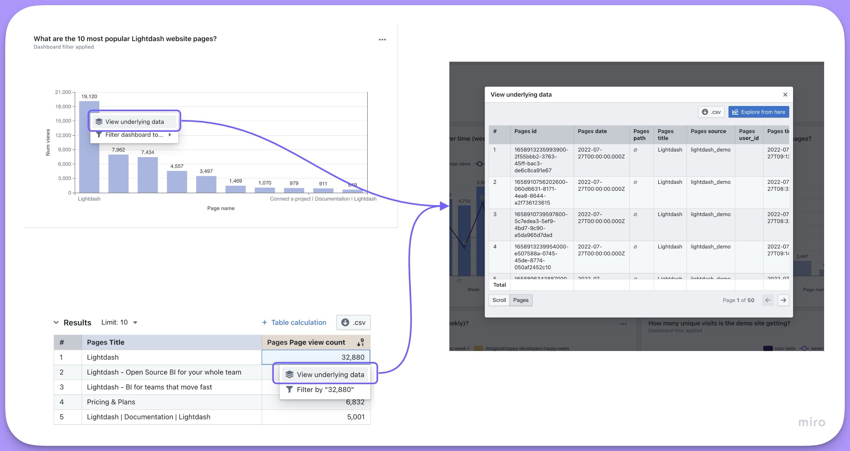
You can limit which dimensions are shown, as well as add metrics to be included, for a field when a user clicks View underlying data by adding the list of dimensions and/or metrics to your .yml files.

When show_underlying_values is not explicitly defined for a metric, View underlying data is capped at the first 50 dimensions from the Table (including joined tables). To show more than 50 dimensions, or to control exactly which fields appear, specify the fields explicitly in show_underlying_values (or default_show_underlying_values at the model level) in your .yml.

Hidden dimensions (with hidden: true) cannot be included in drilldowns. If you need a dimension to appear in drilldowns but not in the Explore sidebar, consider using groups to organize dimensions instead.

models:
  - name: sales_stats
    meta:
      joins:
        - join: web_sessions
          sql_on: ${web_sessions.date} = ${sales_stats.date}
    columns:
      - name: user_id
        description: 'Unique ID for users.'
        meta:
          dimension:
            type: string
          metrics:
            count_users:
              type: count_distinct
              show_underlying_values:
                - revenue_gbp_total_est
                - actual_date
                - web_sessions.session_id # field from joined table

Default show underlying values

You can set a default show_underlying_values configuration at the model level using default_show_underlying_values. This applies to all metrics in that model, and individual metrics can override it by specifying their own show_underlying_values. See default_show_underlying_values in the Tables reference for full details and examples. The list of fields must be made of dimension names (or metrics if you’d like to include them) from the base table or from any joined tables. To reference a field from a joined table, you just need to prefix the field name with the joined table name, like this: my_joined_table_name.my_dimension. The order that the fields are listed in show_underlying_values is the order that they’ll appear in on the view underlying data table.

Referencing time intervals in show underlying values

You can reference specific time intervals of dimensions in the show_underlying_values list. When a dimension has time intervals defined, you can reference the specific interval by appending the interval name to the dimension name (e.g., session_start_month, session_end_quarter).

      count:
        type: count
        show_underlying_values:
          - session_start_month
          - session_end_quarter

In this example, session_start_month and session_end_quarter reference the MONTH and QUARTER time intervals of the session_start and session_end dimensions respectively.

Groups

You can group your dimensions and metrics in the sidebar using the groups parameter. To do this, you need to set up group_details in the model’s configuration. Then, you can use these groups to organize metrics and dimensions. You can create nested groups up to 2 levels.

dbt v1.9 and earlier
dbt v1.10+ and Fusion
Lightdash YAML

models:
  - name: baskets
    meta:
      group_details:
        product_details:
          label: Product Details
          description: 'Fields that have information about the products in the basket.'
        item_details:
          label: Item Details
          description: 'Fields that have information about the items in the basket.'

    columns:
      - name: basket_item_id
        description: 'ID for the product item within the basket.'
        meta:
          dimension:
            groups: ['product_details', 'item_details'] # this would add the dimension to a nested group: `product details` --> `item details`
          metrics:
            count_total_basket_items:
              type: count_distinct
              groups: ['product_details', 'item_details'] # this would add the metric to a nested group: `product details` --> `item details`
      - name: product_name
        description: 'Full name of the product.'
        meta:
          dimension:
            label: 'Product name'
            groups: ['product_details'] # this would add the dimension under the group label: `product_details`
          metrics:
            count_total_product_types:
              type: count_distinct
              groups: ['product_details'] # this would add the metric under the group label: `product_details`

models:
  - name: baskets
    config:
      meta:
        group_details:
          product_details:
            label: Product Details
            description: 'Fields that have information about the products in the basket.'
          item_details:
            label: Item Details
            description: 'Fields that have information about the items in the basket.'

    columns:
      - name: basket_item_id
        description: 'ID for the product item within the basket.'
        config:
          meta:
            dimension:
              groups: ['product_details', 'item_details'] # this would add the dimension to a nested group: `product details` --> `item details`
            metrics:
              count_total_basket_items:
                type: count_distinct
                groups: ['product_details', 'item_details'] # this would add the metric to a nested group: `product details` --> `item details`
      - name: product_name
        description: 'Full name of the product.'
        config:
          meta:
            dimension:
              label: 'Product name'
              groups: ['product_details'] # this would add the dimension under the group label: `product_details`
            metrics:
              count_total_product_types:
                type: count_distinct
                groups: ['product_details'] # this would add the metric under the group label: `product_details`

type: model
name: baskets

group_details:
  product_details:
    label: Product Details
    description: 'Fields that have information about the products in the basket.'
  item_details:
    label: Item Details
    description: 'Fields that have information about the items in the basket.'

dimensions:
  - name: basket_item_id
    description: 'ID for the product item within the basket.'
    groups: ['product_details', 'item_details'] # this would add the dimension to a nested group: `product details` --> `item details`
  - name: product_name
    description: 'Full name of the product.'
    label: 'Product name'
    groups: ['product_details'] # this would add the dimension under the group label: `product_details`

metrics:
  count_total_basket_items:
    type: count_distinct
    sql: ${TABLE}.basket_item_id
    groups: ['product_details', 'item_details'] # this would add the metric to a nested group: `product details` --> `item details`
  count_total_product_types:
    type: count_distinct
    sql: ${TABLE}.product_name
    groups: ['product_details'] # this would add the metric under the group label: `product_details`

Rich text

The richText property allows you to define custom HTML/Markdown templates for displaying metric values in table cells. This enables sophisticated data presentation with formatting, styling, conditional logic, and external integrations.

Rich text only affects UI display in table cells. It has no impact on value formatting, CSV exports, or the underlying data values.

Conditional formatting example

Use Liquid control flow tags for conditional display based on metric values:

dbt v1.9 and earlier
dbt v1.10+ and Fusion
Lightdash YAML

columns:
  - name: customer_lifetime_value
    meta:
      metrics:
        average_clv:
          type: average
          richText: |
            {% raw %}{% if value.raw >= 100 %}
            ### 📈 ${ value.formatted }
            **Excellent** Average CLV
            {% elsif value.raw >= 50 %}
            ### 📊 ${ value.formatted }
            **Good** Average CLV
            {% else %}
            ### ⚠️ ${ value.formatted }
            **Low** Average CLV
            {% endif %}{% endraw %}

columns:
  - name: customer_lifetime_value
    config:
      meta:
        metrics:
          average_clv:
            type: average
            richText: |
              {% raw %}{% if value.raw >= 100 %}
              ### 📈 ${ value.formatted }
              **Excellent** Average CLV
              {% elsif value.raw >= 50 %}
              ### 📊 ${ value.formatted }
              **Good** Average CLV
              {% else %}
              ### ⚠️ ${ value.formatted }
              **Low** Average CLV
              {% endif %}{% endraw %}

metrics:
  average_clv:
    type: average
    sql: ${TABLE}.customer_lifetime_value
    richText: |
      {% raw %}{% if value.raw >= 100 %}
      ### 📈 ${ value.formatted }
      **Excellent** Average CLV
      {% elsif value.raw >= 50 %}
      ### 📊 ${ value.formatted }
      **Good** Average CLV
      {% else %}
      ### ⚠️ ${ value.formatted }
      **Low** Average CLV
      {% endif %}{% endraw %}

Liquid templating in rich text

Use templates to configure values dynamically at runtime based on query results. Available liquid tags

Tag	Description
`${ value.formatted }`	The exact value of the dimension as seen in the Lightdash UI. For example `$1,427.20`
`${ value.raw }`	The raw value of the dimension returned from the underlying SQL query. For example `1427.2`
`${ row.table_name.column_name.formatted }`	The exact value of the column as seen in the Lightdash UI. For example `$1,427.20`
`${ row.table_name.column_name.raw }`	The raw value of the dimension returned from the underlying SQL query. For example `1427.2`

Available liquid filters Filters can be used to make small transformations of your values:

url_encode: Encode a string as URL safe, for example it replaces spaces with %20.
${ value.formatted | url_encode }
downcase: Convert a string to lowercase.
${ value.formatted | downcase }
append: Append one string to another.
${ value.formatted | append: ".html" }

There are many more filters available in the Liquid documentation.

Filters

Filters are applied to metrics any time that metric is used in Lightdash. Filters can only be used with aggregate metric types. For example, we could add a filter to our users count to make sure it didn’t include user IDs with closed accounts, like this:

dbt v1.9 and earlier
dbt v1.10+ and Fusion
Lightdash YAML

models:
  - name: sales_stats
    columns:
      - name: user_id
        description: 'Unique ID for users.'
        meta:
          dimension:
            type: string
          metrics:
            count_users:
              type: count_distinct
              filters:
                - is_closed_account: false

models:
  - name: sales_stats
    columns:
      - name: user_id
        description: 'Unique ID for users.'
        config:
          meta:
            dimension:
              type: string
            metrics:
              count_users:
                type: count_distinct
                filters:
                  - is_closed_account: false

type: model
name: sales_stats

dimensions:
  - name: user_id
    description: 'Unique ID for users.'
    type: string

metrics:
  count_users:
    type: count_distinct
    sql: ${TABLE}.user_id
    filters:
      - is_closed_account: false

These filters do not appear in the Filters tab in the Explore view, instead, they are applied automatically in the SQL query that fetches your results. That means filters added using the filter parameter can’t be removed in the UI and won’t be visible to users unless they look at the SQL query.

Available filter types

Type	Example (in English)	Example (as code)
is	User name is equal to katie	`user_name: "katie"`
is not	User name is not equal to katie	`user_name: "!katie"`
contains	User name contains katie	`user_name: "%katie%"`
does not contain	User name does not contain katie	`user_name: "!%katie%"`
starts with	User name starts with katie	`user_name: "katie%"`
ends with	User name ends with katie	`user_name: "%katie"`
is greater than (number)	Number of orders is greater than 4	`num_orders: "> 4"`
in the past (date) (interval)	Date is before x (days / months / years)	`date: "inThePast 14 months"`
in the next (date) (interval)	Date is after x (days / months / years)	`date: "inTheNext 14 days"`
is greater than or equal to	Number of orders is greater than or equal to 4	`num_orders: ">= 4"`
is less than	Number of orders is less than 4	`num_orders: "< 4"`
is less than or equal to	Number of orders is less than or equal to 4	`num_orders: "<= 4"`
is null	Status is NULL	`status: "null"`
is not null	Status is not NULL	`status: "!null"`
is [boolean]	Is complete is true	`is_complete: "true"`
is not [boolean]	Is complete is false or null	`is_complete: "!true"`

Date filters

For date filtering, use inThePast or inTheNext followed by a number and time unit (days, months, or years). These keywords are case sensitive and must be written exactly as shown.

filters:
  - created_at: 'inThePast 30 days'

Special characters in filters

To use special characters such as %!_> in your filter value you can either put the value in quotes, or escape special characters with a backslash \. For example, if you wanted to filter for subscription status of is_subscribed you can write the metric in one of these ways:

filters:
  - subscription_status: 'is_subscribed'

filters:
  - subscription_status: is\_subscribed

Filtering using a list of values

To filter a field using a list of values you can supply them as an array for that field. This generates a SQL IN clause, e.g. WHERE order_status IN ('completed', 'shipped'). For example, if you wanted to filter for orders with order status completed or shipped you should write the metric like:

dbt v1.9 and earlier
dbt v1.10+ and Fusion
Lightdash YAML

columns:
  - name: order_id
    meta:
      metrics:
        completed_or_shipped_order_count:
          type: count_distinct
          filters:
            - order_status:
                - completed
                - shipped

columns:
  - name: order_id
    config:
      meta:
        metrics:
          completed_or_shipped_order_count:
            type: count_distinct
            filters:
              - order_status:
                  - completed
                  - shipped

type: model
name: my_model

dimensions:
  - name: order_id

metrics:
  completed_or_shipped_order_count:
    type: count_distinct
    sql: ${TABLE}.order_id
    filters:
      - order_status:
          - completed
          - shipped

Filters are joined using `AND`

For example:

filters:
  - is_closed_account: false
  - is_7d_active: true

Would give you logic like is_closed_account = TRUE AND is_7d_active = FALSE.

Adding filters from joined models

To filter using a field from a joined model, just use the syntax model_name.field, like this:

dbt v1.9 and earlier
dbt v1.10+ and Fusion
Lightdash YAML

models:
  - name: sales_stats
    meta:
      joins:
        - join: web_sessions
          sql_on: ${web_sessions.date} = ${sales_stats.date}
    columns:
      - name: user_id
        description: 'Unique ID for users.'
        meta:
          dimension:
            type: string
          metrics:
            count_users:
              type: count_distinct
              filters:
                - is_closed_account: false
                - web_sessions.is_bot_user: false

models:
  - name: sales_stats
    config:
      meta:
        joins:
          - join: web_sessions
            sql_on: ${web_sessions.date} = ${sales_stats.date}
    columns:
      - name: user_id
        description: 'Unique ID for users.'
        config:
          meta:
            dimension:
              type: string
            metrics:
              count_users:
                type: count_distinct
                filters:
                  - is_closed_account: false
                  - web_sessions.is_bot_user: false

type: model
name: sales_stats

joins:
  - join: web_sessions
    sql_on: ${web_sessions.date} = ${sales_stats.date}

dimensions:
  - name: user_id
    description: 'Unique ID for users.'
    type: string

metrics:
  count_users:
    type: count_distinct
    sql: ${TABLE}.user_id
    filters:
      - is_closed_account: false
      - web_sessions.is_bot_user: false

Referencing time intervals in filters

You can reference specific time intervals of dimensions in metric filters. When a dimension has time intervals defined, you can filter on the specific interval by appending the interval name to the dimension name (e.g., session_start_day).

      count:
        type: count
        filters:
          - session_start_day: "!null"

In this example, the filter checks that session_start_day (the DAY time interval of the session_start dimension) is not null.

Metric filters cannot be used with non-aggregate metrics

You can’t use filters with non-aggregate metric types. Instead, if your non-aggregate metrics are referencing aggregate metric types, you need to apply metric filters to the aggregate metrics. Here’s an example: imagine you wanted to calculate the average cost per item that had the status shipped. You would need to do something like this in your .yml:

dbt v1.9 and earlier
dbt v1.10+ and Fusion
Lightdash YAML

models:
  - name: orders
    meta:
      metrics:
        average_cost_per_item_shipped:
          type: number
          sql: ${total_cost_of_shipped} / ${count_unique_items_shipped}
    columns:
      - name: item_id
        description: 'Unique ID for items ordered.'
        meta:
          dimension:
            type: string
          metrics:
            count_unique_items:
              type: count_distinct
            count_unique_items_shipped:
              type: count_distinct
              filters:
                - status: 'shipped'
      - name: item_cost
        description: 'Cost for each item ordered.'
        meta:
          dimension:
            type: number
          metrics:
            total_cost:
              type: sum
            total_cost_of_shipped:
              type: sum
              filters:
                - status: 'shipped'

models:
  - name: orders
    config:
      meta:
        metrics:
          average_cost_per_item_shipped:
            type: number
            sql: ${total_cost_of_shipped} / ${count_unique_items_shipped}
    columns:
      - name: item_id
        description: 'Unique ID for items ordered.'
        config:
          meta:
            dimension:
              type: string
            metrics:
              count_unique_items:
                type: count_distinct
              count_unique_items_shipped:
                type: count_distinct
                filters:
                  - status: 'shipped'
      - name: item_cost
        description: 'Cost for each item ordered.'
        config:
          meta:
            dimension:
              type: number
            metrics:
              total_cost:
                type: sum
              total_cost_of_shipped:
                type: sum
                filters:
                  - status: 'shipped'

type: model
name: orders

dimensions:
  - name: item_id
    description: 'Unique ID for items ordered.'
    type: string
  - name: item_cost
    description: 'Cost for each item ordered.'
    type: number

metrics:
  count_unique_items:
    type: count_distinct
    sql: ${TABLE}.item_id
  count_unique_items_shipped:
    type: count_distinct
    sql: ${TABLE}.item_id
    filters:
      - status: 'shipped'
  total_cost:
    type: sum
    sql: ${TABLE}.item_cost
  total_cost_of_shipped:
    type: sum
    sql: ${TABLE}.item_cost
    filters:
      - status: 'shipped'
  average_cost_per_item_shipped:
    type: number
    sql: ${total_cost_of_shipped} / ${count_unique_items_shipped}

Level of detail metrics

When you build a query in Lightdash, every metric in the results is grouped by the dimensions you’ve selected. This is usually what you want, but sometimes you need a metric to be calculated at a different granularity than the rest of the query. For example, you might want a denominator that stays at a coarser grain even when you add more dimensions to the view. This is commonly known as a “level of detail” (LOD) calculation. The idea is that certain metrics should ignore specific dimensions during aggregation, so their values remain stable regardless of how the data is sliced. Coming to the demo site soon.

The problem

This comes up most often with percentage or ratio metrics. Consider this scenario: you want to calculate “what % of accounts in each segment have Won deals?” and you want to break this down by deal plan. The numerator (accounts with Won deals) should naturally vary by plan. But the denominator (total accounts in the segment) should not. There are 152 Enterprise accounts regardless of which plan you’re analyzing. When you join accounts to deals and group by both segment and plan, the denominator gets scoped to only the accounts that have deals in that plan. This is the default behavior in any BI tool that uses a join-then-group approach. Without level of detail (denominator grouped by plan):

Segment	Plan	Accounts with Won Deals	Total Accounts	%
Enterprise	Basic	36	107	33.6%
Enterprise	Professional	13	46	28.3%

The total accounts column shows 107 and 46 because only accounts that have deals in that specific plan are included in the count. With level of detail (denominator independent of plan):

Segment	Plan	Accounts with Won Deals	Total Accounts	%
Enterprise	Basic	36	152	23.7%
Enterprise	Professional	13	152	8.6%

The total accounts column stays at 152 because the denominator is computed independently of the plan dimension. This is achieved by pre-computing the denominator in a separate CTE in your dbt model.

The workaround

The solution is to pre-compute the coarser-grain metric (total accounts per segment) in your dbt model, so it is always correct regardless of which dimensions are selected in Lightdash. Step 1: Pre-compute the denominator in your dbt model

SQL model

with segment_totals as (
    select
        segment,
        count(distinct account_id) as total_accounts_in_segment
    from {{ ref('accounts') }}
    group by segment
),

account_deals as (
    select
        a.account_id,
        a.segment,
        d.deal_id,
        d.plan,
        d.stage
    from {{ ref('accounts') }} a
    inner join {{ ref('deals') }} d on a.account_id = d.account_id
)

select
    ad.*,
    st.total_accounts_in_segment
from account_deals ad
left join segment_totals st on ad.segment = st.segment

Step 2: Define the metrics in your YAML

dbt v1.9 and earlier
dbt v1.10+ and Fusion
Lightdash YAML

models:
  - name: account_deal_metrics
    meta:
      metrics:
        pct_accounts_with_won_deals:
          type: number
          label: "% Accounts with Won Deals"
          format: percent
          sql: ${unique_accounts_with_won_deals} / NULLIF(${segment_total_accounts}, 0)
    columns:
      - name: account_id
        meta:
          dimension:
            type: string
            hidden: true
          metrics:
            unique_accounts_with_won_deals:
              type: count_distinct
              filters:
                - stage: 'Won'
      - name: segment
        meta:
          dimension:
            type: string
      - name: plan
        meta:
          dimension:
            type: string
      - name: total_accounts_in_segment
        meta:
          dimension:
            type: number
          metrics:
            segment_total_accounts:
              type: max

models:
  - name: account_deal_metrics
    config:
      meta:
        metrics:
          pct_accounts_with_won_deals:
            type: number
            label: "% Accounts with Won Deals"
            format: percent
            sql: ${unique_accounts_with_won_deals} / NULLIF(${segment_total_accounts}, 0)
    columns:
      - name: account_id
        config:
          meta:
            dimension:
              type: string
              hidden: true
            metrics:
              unique_accounts_with_won_deals:
                type: count_distinct
                filters:
                  - stage: 'Won'
      - name: segment
        config:
          meta:
            dimension:
              type: string
      - name: plan
        config:
          meta:
            dimension:
              type: string
      - name: total_accounts_in_segment
        config:
          meta:
            dimension:
              type: number
            metrics:
              segment_total_accounts:
                type: max

type: model
name: account_deal_metrics

dimensions:
  - name: account_id
    type: string
    hidden: true
  - name: segment
    type: string
  - name: plan
    type: string
  - name: total_accounts_in_segment
    type: number

metrics:
  unique_accounts_with_won_deals:
    type: count_distinct
    sql: ${TABLE}.account_id
    filters:
      - stage: 'Won'
  segment_total_accounts:
    type: max
    sql: ${TABLE}.total_accounts_in_segment
  pct_accounts_with_won_deals:
    type: number
    label: "% Accounts with Won Deals"
    format: percent
    sql: ${unique_accounts_with_won_deals} / NULLIF(${segment_total_accounts}, 0)

The key insight is that total_accounts_in_segment is pre-computed in the SQL and is the same value for every row in a segment. Using max as the aggregation returns the correct segment-level total, regardless of what other dimensions (like plan) are in the query. The pct_accounts_with_won_deals metric then divides the numerator (which correctly varies by plan) by the denominator (which stays fixed per segment).

​Adding metrics to your project using the meta tag.

​1. Using the column meta tag

​2. Using the model meta tag

​Metric Categories

​Aggregate metrics

​Non-aggregate metrics

​Post calculation metrics

​Metric configuration

​Metric types

​percentile

​median

​average

​boolean

​count

​count_distinct

​date

​max

​min

​number

​sum

​sum_distinct

​average_distinct

​string

​percent_of_previous

​percent_of_total

​running_total

​Description

​Format

​Example format expressions

​Format (legacy)

​Round (legacy)

​Compact

​Separator

​Custom SQL in aggregate metrics

​Referencing time intervals in custom SQL

​Using custom SQL in non-aggregate metrics

​Show underlying values

​Default show underlying values

​Referencing time intervals in show underlying values

​Groups

​Rich text

​Conditional formatting example

​Liquid templating in rich text

​Filters

​Available filter types

​Date filters

​Special characters in filters

​Filtering using a list of values

​Filters are joined using AND

​Adding filters from joined models

​Referencing time intervals in filters

​Metric filters cannot be used with non-aggregate metrics

​Tags

​Level of detail metrics

​The problem

​The workaround

Adding metrics to your project using the `meta` tag.

1. Using the column `meta` tag

2. Using the model `meta` tag

Metric Categories

Aggregate metrics

Non-aggregate metrics

Post calculation metrics

Metric configuration

Metric types

percentile

median

average

boolean

count

count_distinct

date

max

min

number

sum

sum_distinct

average_distinct

string

percent_of_previous

percent_of_total

running_total

Description

Format

Example format expressions

Format (legacy)

Round (legacy)

Compact

Separator

Custom SQL in aggregate metrics

Referencing time intervals in custom SQL

Using custom SQL in non-aggregate metrics

Show underlying values

Default show underlying values

Referencing time intervals in show underlying values

Groups

Rich text

Conditional formatting example

Liquid templating in rich text

Filters

Available filter types

Date filters

Special characters in filters

Filtering using a list of values

Filters are joined using `AND`

Adding filters from joined models

Referencing time intervals in filters

Metric filters cannot be used with non-aggregate metrics

Tags

Level of detail metrics

The problem

The workaround